Granger Causality and Hypothesis Testing

This article discusses causal illusions as a form of cognitive bias and explores the use of Granger causality to detect causal structures in time series. It is common practice to analyse (linear) structure, estimate linear models and perform forecasts based on single stationary time series. However, the world does not consist of independent stochastic processes. In accordance with general equilibrium theory, economists usually assume that everything depends on everything else. Therefore, it is important to understand and quantify the (causal) relationships between different time series.

Epiphenomena

Epiphenomena is a class of causal illusions where the direction of causal relationships is ambiguous. For example, when you spend time on the bridge of a ship with a large compass in front, you can easily develop the impression that the compass is directing the ship rather than merely reflecting its direction. Here is an image that perfectly illustrates the point that correlation is not causation:

Nassim Nicholas Taleb explored this concept in his book Antifragile to highlight the causal illusion that universities generate wealth in society. He presented a miscellany of evidence which suggests that classroom education does not lead to wealth as much as it comes from wealth (an epiphenomenon). Taleb proposes that antifragile risk-taking is largely responsible for innovation and growth instead of education and formal, organized research. However, it does not mean that theories and research play no role, but rather shows that we are fooled by randomness into overestimating the role of good-sounding ideas. Because of cognitive biases, historians are prone to epiphenomena and other illusions of cause and effect.

We can debunk epiphenomena in the cultural discourse and consciousness by looking at the sequence of events and checking their order or occurrences. This method is refined by Clive Granger who developed a rigorously scientific approach that can be used to establish causation by looking at time series sequences and measuring the "Granger cause".

Granger causality

In the following, we present the definition of Granger causality and the different possibilities of causal events resulting from it. Consider two weakly stationary time series $x$ and $y$:

1. Granger Causality: $x$ is (simply) Granger causal to $y$ if and only if the application of an optimal linear prediction function leads to a smaller forecast error variance on the future value of $y$ if current and past values of $x$ are used.

2. Instantaneous Granger Causality: $x$ is instantaneously Granger causal to $y$ if and only if the application of an optimal linear prediction function leads to a smaller forecast error variance on the future value of $y$ if the future value of $x$ is used in addition to the current and past values of $x$.

3. Feedback: There is feedback between $x$ and $y$ if $x$ is causal to $y$ and $y$ is causal to $x$. Feedback is only defined for the case of simple causal relations.

Hypothesis testing in general linear models

Consider the general linear model $\mathbf{Y} = X \boldsymbol{\beta} + \varepsilon$. In hypothesis testing, we want to know whether certain variables influence the result. If, say, the variable $x_1$ does not influence $\mathbf{Y}$, then we must have $\beta_1 = 0$. So the goal is to test the hypothesis $H_0: \beta_1 = 0$ versus $H_1: \beta_1 \neq 0$. We will tackle a more general case, where $\beta$ can be split into two vectors $\beta_0$ and $\beta_1$, and we test if $\beta_1$ is zero.

Suppose $\underset{n \times p}{X} = \left(\underset{n \times p_0}{X_0} \underset{n \times\left(p - p_0\right)}{X_1}\right)$ and $\boldsymbol{\beta} = \left(\begin{array}{c}\boldsymbol{\beta}_0 \\ \boldsymbol{\beta}_1\end{array}\right)$, where $\operatorname{rank}(X)= p$, $\operatorname{rank}\left(X_0\right) = p_0$. We want to test $H_0: \boldsymbol{\beta}_1 = 0$ against $H_1: \boldsymbol{\beta}_1 \neq 0$. Under $H_0$, $X_1 \boldsymbol{\beta}_1$ vanishes and

Under $H_0$, the maximum likelihood estimation (MLE) of $\boldsymbol{\beta}_0$ and $\sigma^2$ are

and we have previously shown these are independent. So the fitted values under $H_0$ are

where $P_0=X_0\left(X_0^T X_0\right)^{-1} X_0^T$.

Note that our poor estimators wear two hats instead of one. We adopt the convention that the estimators of the null hypothesis have two hats, while those of the alternative hypothesis have one.

The generalized likelihood ratio test of $H_0$ against $H_1$ is

We reject $H_0$ when $2 \log \Lambda$ is large, equivalently when $\frac{\mathrm{RSS}_0-\mathrm{RSS}}{\mathrm{RSS}}$ is large. Under $H_0$, we have

which is approximately a $\chi_{p-p_0}^2$ random variable. We can also get an exact null distribution, and get an exact test. The F statistic under $H_0$ is given by

Hence we reject $H_0$ if $F > F_{p-p_0, n-p}(\alpha)$. $\mathrm{RSS}_0 -\mathrm{RSS}$ is the reduction in the sum of squares due to fitting $\boldsymbol{\beta}_1$ in addition to $\boldsymbol{\beta}_0$.

Source of var.	d.f.	sum of squares	mean squares
Fitted model	$p - p_0$	$\mathrm{RSS}_0-\mathrm{RSS}$	$\frac{\mathrm{RSS}_0-\mathrm{RSS}}{p - p_0}$
Residual	$n - p$	$\mathrm{RSS}$	$\frac{\mathrm{RSS}}{n - p}$
Total	$n - p_0$	$\mathrm{RSS}_0$

The ratio $\frac{\mathrm{RSS}_0-\mathrm{RSS}}{\mathrm{RSS}_0}$ is sometimes known as the proportion of variance explained by $\boldsymbol{\beta}_1$, and denoted $R^2$.

def fit(data, p=1):
    n = data.shape[0] - p
    Y = data[p:]
    X = np.stack([np.ones(n)] + [data[p-i-1:-i-1] for i in range(p)], axis=-1)
    
    beta_mle = np.linalg.inv(X.T.dot(X)).dot(X.T.dot(Y))
    R = Y - X.dot(beta_mle)
    RSS = R.T.dot(R) 
    var_mle = RSS / n
    
    return beta_mle, var_mle, RSS

Causality tests

To test for simple causality from $x$ to $y$, it is examined whether the lagged values of $x$ in the regression of $y$ on lagged values of $x$ and $y$ significantly reduce the error variance. By using the ordinary least squares (OLS) method, the following equation is estimated:

with $k_0 = 1$. An F test is applied to test the null hypothesis, $H_0: \alpha^{1}_{12} = \alpha^{1}_{12} = \cdots = \alpha^{k_2}_{12} = 0$. By changing $x$ and $y$, it can be tested whether a simple causal relation from $y$ to $x$ exists. There is a feedback relation if the null hypothesis is rejected in both directions. To test whether there is instantaneous causality, we finally set $k_0 = 0$ and perform a t or F test for the null hypothesis $H_0: \alpha^{0}_{12} = 0$.

def causality_tests(y, x, alpha=0.05, k_1=1, maxlag=1):
    for k_2 in range(1, maxlag + 1):
        p = 1 + k_1 + k_2
        n = y.shape[0] - np.max([k_1, k_2])

        _, _, RSS = fit_xy(y, x, k_1, k_2)
        _, _, RSS_0 = fit(y, k_1)

        chi2 = n * np.log(RSS_0 / RSS)
        f = ((RSS_0 - RSS) / k_2) / (RSS / (n - p))

One problem with this test is that the results are strongly dependent on the number of lags of the explanatory variable, $k_2$. There is a trade-off: the more lagged values we include, the better the influence of this variable can be captured. This argues for a high maximal lag. On the other hand, the power of this test is lower the more lagged values are included.

We can fit a linear model on real financial data and use the Granger causality test to find causal relationships.

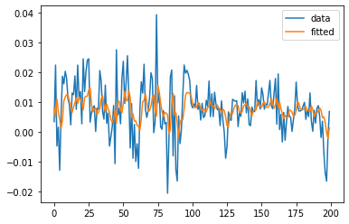
Hypothesis Test (p=1)
F test:       F=24.4610 , p=0.0000, df_denom=199, df_num=1
chi2 test: chi2=23.3023 , p=0.0000, df=1
Reject null hypothesis

Hypothesis Test (p=2)
F test:       F=8.2501  , p=0.0045, df_denom=197, df_num=1
chi2 test: chi2=8.2051  , p=0.0042, df=1
Reject null hypothesis

Hypothesis Test (p=3)
F test:       F=0.4181  , p=0.5187, df_denom=195, df_num=1
chi2 test: chi2=0.4262  , p=0.5139, df=1
Accept null hypothesis

Hypothesis Test (p=4)
F test:       F=4.9506  , p=0.0272, df_denom=193, df_num=1
chi2 test: chi2=5.0148  , p=0.0251, df=1
Reject null hypothesis