Black Scholes Model with Stock Simulation

The article explores the use of geometric Brownian Motion (GBM) to simulate the price of stocks. The concept naturally extends to the Black-Scholes-Merton (BSM) model which is widely used to estimate the pricing variation of financial instruments such as an options contract. Monte Carlo simulation (MCS) is then used to estimate the stock pricing and validate the model predictions.

Geometric Brownian Motion

Stochastic process

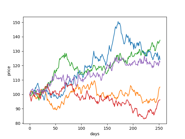
A geometric Brownian motion (GBM) is a continuous-time stochastic process in which the logarithm of the randomly varying quantity follows a Brownian motion (also called a Wiener process) with drift. The stock price $S_t$ is said to follow a GBM if it satisfies the following stochastic differential equation (SDE):

dS_t = \mu S_t dt + \sigma S_t dW_t

$W_t$ is a Wiener process or Brownian motion, and the expected return $\mu$ and the standard deviation of returns (volatility) $\sigma$ are constants. We also assume the stock does not pay any dividends, there are no transaction costs and the continuously compounding interest rate is $r > 0$ . Note that $W_t$ is normally distributed with mean $0$ and variance $t$ . For an arbitrary initial value $S_0$ the above SDE has the analytic solution:

S_t = S_0 \exp \left[ \left( \mu - \frac{\sigma^2}{2} \right) t + \sigma W_t \right]

The GBM is technically a Markov process. The stock price hence follows a random walk and is consistent with the weak form of the efficient market hypothesis (EMH).

# Calculate stock price at time t
S = S0 * np.exp(r * t - 1/2 * sigma**2 * t + sigma * np.random.randn() * np.sqrt(t))

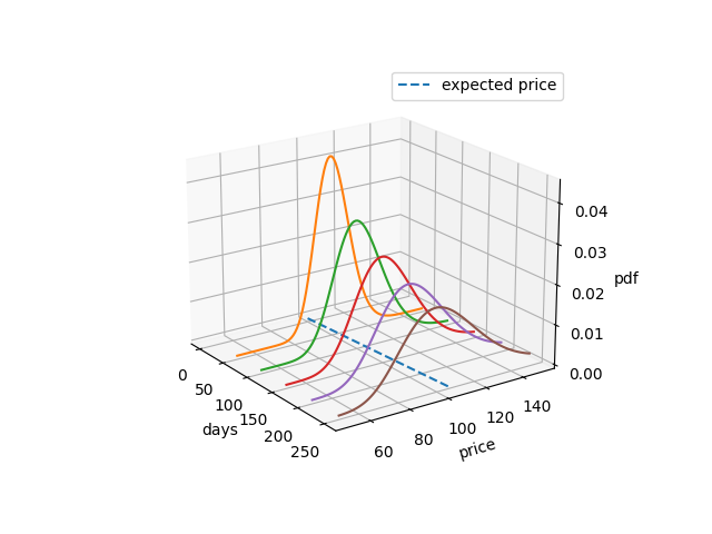
Probability density function

Since the exponent of $S_t$ is normally distributed, we can use the change of variable formula to calculate the probability distribution of $S_t$ . Note that for $S_t$ the exponent is normally distributed with mean $\ln S_0 + \left( \mu - \frac{\sigma^2}{2} \right) t$ and variance $\sigma^2 t$ . Hence, $S_t$ follows a log-normal distribution:

S_t \sim \mathcal{LN} \left[\ln S_0 + \left( \mu - \frac{\sigma^2}{2} \right) t, \sigma^2 t\right]

Maximum likelihood estimate

In order to estimate the percentage drift $\mu$ and percentage volatility $\sigma$ , we use the previously calculated probability density function for log-normal distribution to obtain an expression for the log-likelihood:

\begin{aligned} L =& - \frac{n}{2} \ln v - \frac{n}{2} \ln 2\pi - \sum_{i=1}^n \ln x_i\\ & - \sum_{i=1}^n -\frac{(\ln x_i -m)^2}{2 v} \end{aligned}

Differentiate with respect to the model parameters to find the maximum likelihood (ML) estimate:

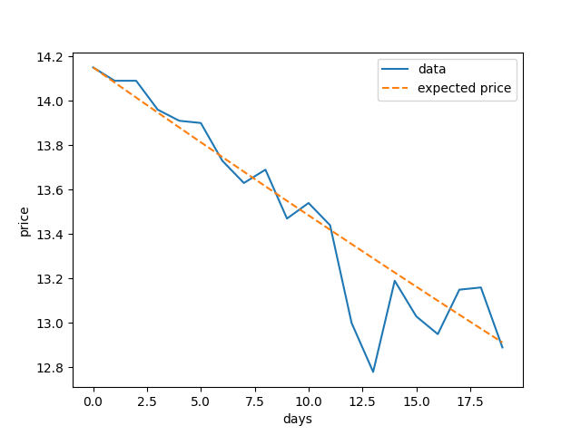
m = \frac{\sum_{i=1}^n \ln x_i}{n}, \quad v = \frac{\sum_{i=1}^n (\ln x_i - m)^2}{n}

We can use the GBM to model real financial data by looking at the General Electric stock daily data over 20 business days.

             High    Low   Open  Close      Volume  Adj Close
Date                                                         
2021-06-01  14.34  14.10  14.23  14.15  50276900.0  14.139239
2021-06-02  14.18  14.01  14.18  14.09  39936800.0  14.079286
2021-06-03  14.37  13.94  13.99  14.09  63163800.0  14.079286
2021-06-04  14.20  13.86  14.16  13.96  64071200.0  13.949385
2021-06-07  14.07  13.86  14.00  13.91  37349100.0  13.899423

By calculating the mean and variance of the log returns, we can obtain an estimate of the risk free interest rate and volatility.

Black Scholes Model

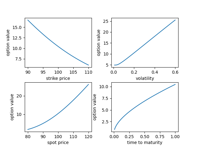
The Black-Scholes Formula

The Black-Scholes call option formula is calculated by multiplying the stock price $S_t$ by the cumulative standard normal distribution. Thereafter, the net present value (NPV) of the strike price $K$ with risk-free interest rate $r$ and time to maturity $t$ is multiplied by the cumulative standard normal distribution and subtracted from the resulting value. The call option price $C$ is therefore given by:

C = S_t N(d_1) - K e^{-rt} N(d_2)

$N(d_2)$ is the risk-adjusted probability that the option will be exercised. $N(d_1)$ is the factor by which the present value of contingent receipt of the stock exceeds the current stock price.

d_1 = \frac{\ln \frac{S_t}{K} + \left( r + \frac{\sigma^2}{2} \right)t}{\sigma \sqrt{t}}, \quad d_2 = d_1 - \sigma \sqrt{t}

To price a derivative in the Black-Scholes world, we must do so under a measure which does not allow arbitrage (clearly the existence of arbitrage in any model is cause for concern). Such a measure is called a risk-neutral measure.

# Calculate the value of a call option using the Black-Scholes formula
d1 = (1 / sigma * np.sqrt(t)) * (np.log(S0/K) + (r + 1/2 * sigma**2 * t))
d2 = d1 - sigma * np.sqrt(t)
C = S0 * (norm.cdf(d1)) - np.exp(-r * t) * K * norm.cdf(d2)

Monte Carlo for vanilla option

Options are financial instruments that give the holder the right, but not the obligation, to buy or sell an underlying asset at a predetermined price within a given timeframe. A vanilla option is a call option or put option that has no special or unusual features. For a call option with strike $K > 0$ , the payoff at time $T$ is given by:

\max (S_T - K, 0)

We can compare the average payoff of an option simulated with GBM with its price calculated using the Black-Scholes model.

# Monte Carlo simulation
for i in range(NUM_SIMS):
    stock_price = S0 * np.exp(r * t - 1/2 * sigma**2 * t + sigma * np.random.randn() * np.sqrt(t))
    payoff[i] = (stock_price - K) * np.exp(-r * t) if stock_price > K else 0